


Document Actions
gvSIG-Desktop 1.10. User Manual
- Documents
- 2D views
- Vectorial tools
- Raster tools
- Introduction
- Layer properties
- Layer information
- Raster properties
- Setting a visible scale range for a layer
- Enhancement (Raster properties)
- Image statistics
- Bands and files selector
- Transparency per pixel
- General components
- Table of contents (ToC)
- Properties of a view in gvSIG
- Maps
- Copying layers in gvSIG
- Deleting layers
- Exporting to image
Documents
2D views
Vectorial tools
Introduction
Views are the gvSIG documents used as the working area of cartographic information.
A view can contain different layers of geographic information (hydrography, transport infrastructures, administrative regions, contour lines, etc.).
When one of the views that make up a project is opened, a new window appears divided into the following parts:
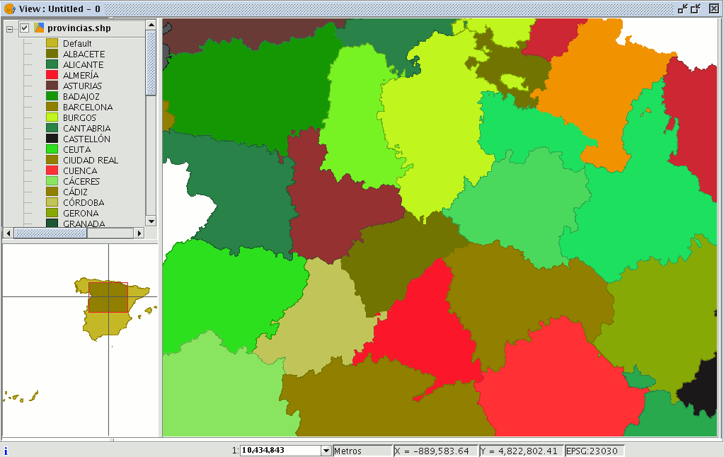
Table of contents (ToC): The ToC is located on the left-hand side of the window. The Table of Contents lists all the layers it contains and the symbols used to represent the elements which make up the layer.
Display window: The display window is located on the right-hand side of the screen. The project’s cartographic data are shown in this display window.
Locator: The locator is situated in the bottom left-hand corner. The locator allows the current frame to be situated in the work area as a whole.
When a view is opened, the main window increases the number of menus and buttons, thus adding the tools required to work with the elements which make up the view.
The size of the ToC can be enlarged to show a full description of all the themes by simply dragging its edge to the right or downwards.
Layer properties
Introduction
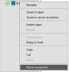
You can access the active layer's properties from its contextual menu (right click on the layer).
General properties
Right click on the selected layer in the ToC to access the properties window.
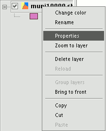
When you click on the “Properties” option, a new dialogue box opens. This can be used to edit some properties.
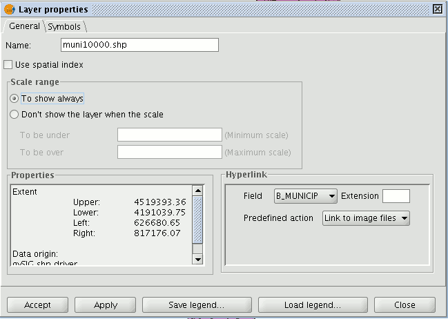
The layer name can be changed by writing the new name in the text field in the “General” tab.
If you wish to rename the selected layer, right click on the layer and go to the "Rename" option.
A new window appears:
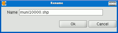
Write the new name in the text field and click on “Ok”.
N.B.: When you do this, the layer name changes in the ToC, but the file name is not changed.
If you mark the “Use spatial index” check box, a spatial index will be created which makes the layer loaded in the view appear more quickly. This is because the view is loaded using this index.
If there are write permissions, a .qix file is created with the same name as the layer it is associated with in the layer’s original directory. If there are no write permissions, the file will be created in the user’s temporary file directory.
A viewing scale range (maximum and minimum) can be set in the properties window.
The file extension and path are shown in the actual properties section.
Raster tools
Introduction
You can access the active layer's properties from its contextual menu (right click on the layer).
Layer properties
Layer information
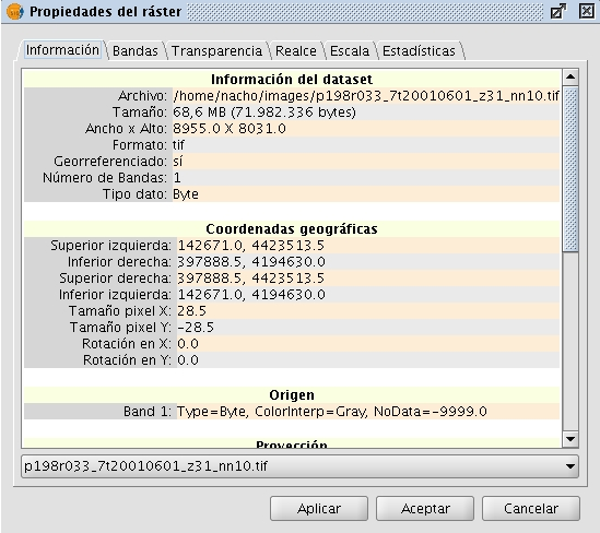
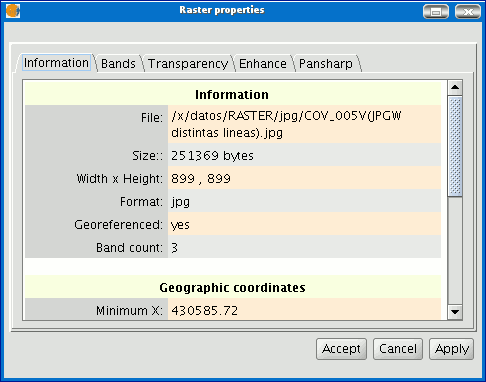
You can find information about the current raster layer through the option "Raster Properties", which shows a dialog with multiple tabs containing information about the raster layer. To get information about the layer, click the tab "Information".
The "Raster Properties" dialog can be accessed in two ways: by right-clicking on the raster layer in the Table of Contents or through the raster properties icon in the toolbar:

Raster Properties icon
Here, set the left button to Raster Layer and select the option Raster Properties from the pull-down button on the right. Make sure that the name of the raster layer for which you want to see information is displayed as current layer in the text box.
The Information tab of the Raster Properties window shows general information about the raster layer. Since a layer can consist of multiple files with the same geographic extension, you can choose the file for which you want to see information from the pull-down tool on the bottom of the "Information" tab window. The information is divided in thematic blocs with a header in bold letters indicating the bloc theme.
The bloc Dataset information shows the name of the file, disk size, width and height in pixels, data format (file extension), whether it is georeferenced, the number of bands and the data type.
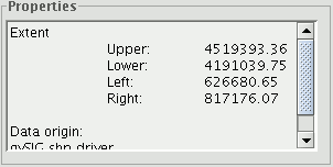
The bloc Geographic coordinates shows the georeferencing information of the layer as well as the pixel size.
The bloc Origin will show an entry for each band in the file. For every band you can see the data type, the colour interpretation and the value that is assigned to NoData pixels. The colour interpretation of a band is important for the display on screen. If a band has an interpretation such as Red, this means that gvSIG will interpret this band to be displayed as the red band in RGB visualization. This colour interpretation will be used as default for the displaying of the image. A band may have the following types of representations: Red, Green, Blue, Gray, Undefined or Alpha. The NoData information associated with the band will not be taken into account when processing the image, and the NoData values can be shown as transparent if needed (see the section "NoData values").
The bloc Projection will show the projection information of the layer, if available. The representation format is WKT.
The bloc Metadata will show metadata information from the image header if available.
Raster Properties. Metadata
Raster properties
Right click on a raster layer and select the "Raster properties" option. This opens a menu in which we can carry out various operations on the raster layer.
This menu is divided into five tabs:
Information: Provides general information about the raster layer, the file path, the number of bands, the pixel dimensions, the file format, the data type and the geographic coordinates of the corners.
Bands: Provides tools to change the mode in which each image band is viewed. Transparency: Provides tools to change the transparency levels that can be applied to a raster layer.
Enhance: Provides a tool to enhance the raster layer. Pansharpening: Provides a tool to increase the satellite image resolution if the panchromatic band for these images is available.
In the “Bands” tab you can make compositions using the different bands in a raster image. You can also add more bands from other files. This is useful when working with Landsat-type images, in which each band is delivered in a different file.
In addition to the “Transparency” option in gvSIg version 0.3, which is now called “opacity”, and which indicates the "occlusion” percentage of this layer over the previous ones, there is now a transparency option which allows the indicated colour groups (RGB) to be completely transparent. This is very useful to eliminate visual artefacts as a result of missing data in orthophotos or satellite images and to remove borders in an image mosaic.
To access the options, click on the corresponding “Activate” check boxes.
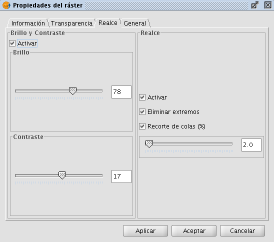
The “Enhance” tab can be used to modify the image brightness, contrast and enhancement. This last option is essential to be able to view 16-bits per band images correctly.
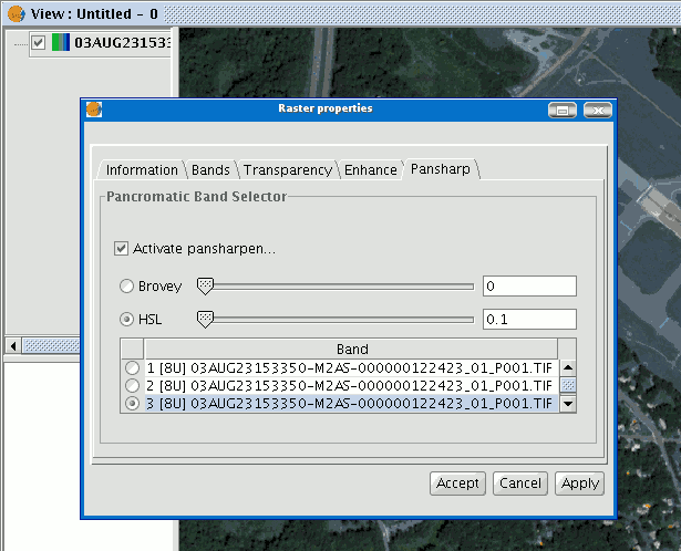
The “Pansharpening” tab can be used to increase the resolution of satellite images if the panchromatic band for these images is available. N.B.: If the image bands are in different files, they must be added to the layer using the “Bands” tab.
Use the “Bands” tab to find the best band combination for the view. In this section, you can load the image which corresponds to the panchromatic band but you must not select it to be visualised.
When the bands have been loaded, you can carry out the pansharpening. Go to the “Pansharpening” tab and activate it by clicking on the “Activate Pansharpening” check box. Select the panchromatic band with which the pansharpening is to be carried out from the band list. Finally, select an algorithm to be applied. There are two methods available, “Brovey” and “HSL”. Both of them have a slide bar control to carry out adjustments.
In “Brovey” the general brightness of the resulting image is increased or decreased.
In “HSL” the coefficient which is added to the brightness taken from the pansharpening band varies before it is replaced in the output image. This coefficient can vary between 0.15 and 0.5. When modified, the obtained result also influences the output image’s general brightness. If you click on the "Apply" or “Ok" buttons, the pansharpening will be applied on the image in the view, thus increasing the image resolution.
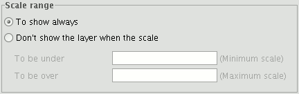
Setting a visible scale range for a layer
To set the layer visibility according to scale range, you can specify the scale ranges in the "General" tab of the Raster Properties window.
The "Raster Properties" dialog can be accessed in two ways: by right-clicking on the raster layer in the Table of Contents, or through the Raster Properties icon in the toolbar:

Raster Properties icon
In the "General" tab, the scale ranges can be set as shown in the picture below:
Raster Properties. Configure Scale ranges
There are two ways to hide the image according to its scale:
- Hide when the scale is bigger than 1:xxx, where xxx is a numeric value to be entered. This corresponds to the minimum scale.
- Hide when the scale is smaller than 1:xxx, where xxx is a numeric value to be entered. This corresponds to the maximum scale.
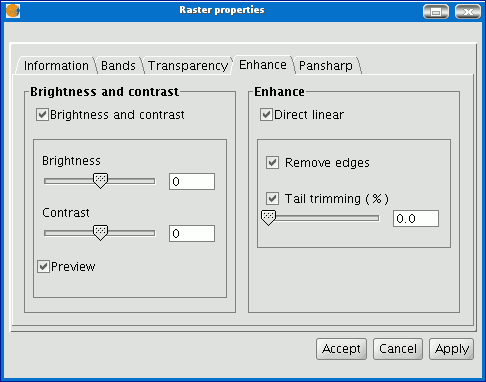
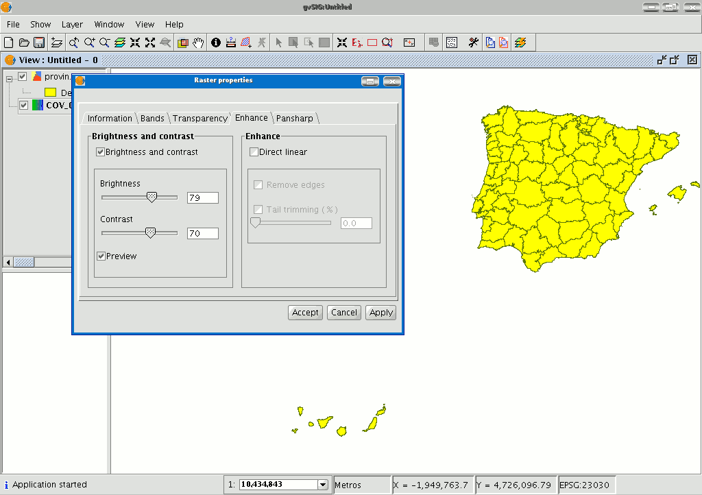
Enhancement (Raster properties)
The Raster Properties dialog contains options for the enhancement of raster layers. The "Raster Properties" dialog can be accessed in two ways: by right-clicking on the raster layer in the Table of Contents or through the raster properties icon in the toolbar:

Raster Properties icon
Here, set the left button to Raster Layer and select the option Raster Properties from the pull-down button on the right. Make sure that the name of the raster layer for which you want to see information is displayed as current layer in the text box.
In the Raster Properties dialog, select the "Enhancement" tab.
Raster Properties. Enhancement
Every modification in this Enhancement dialog will be applied to the current view for visual interpretation purposes and can not be saved as a new layer. If you want to save the enhancements, you will need to use the Filter dialog or the Radiometric Enhancement dialog, depending on whether you want to modify the brightness and contrast or apply a linear enhancement.
On the left side of the dialog, the controls for modifying brightness and contrast are shown. By default, these controls are disabled but if you want to change the values, you can activate them by ticking the "Activate" check box. Then, use the slide bar to alter the slide bar or type the value directly in the corresponding text box.
The right side of the dialog is used for linear enhancement. This is a simplification of linear radiometric enhancement to control the display of images of data types other than Byte. For Byte images, this control is disabled by default. For other data types, these values are automatically set when the raster layer is loaded. It is recommended to use this control only to modify automatically assigned values. For more enhancement options it is more appropriate to use the Radiometric Enhancement function.
The enhancement stretches the data over a range from 0 to 255 to improve visual interpretation. The option "Remove edges" will ignore the minimum and maximum values that appear in the image. The option "Clipping tail (%)" will sort the values from low to high, and cut off the values that are lower or higher than a specified percentage of the total number of values. The effect is a shift in the maximum and minimum values.
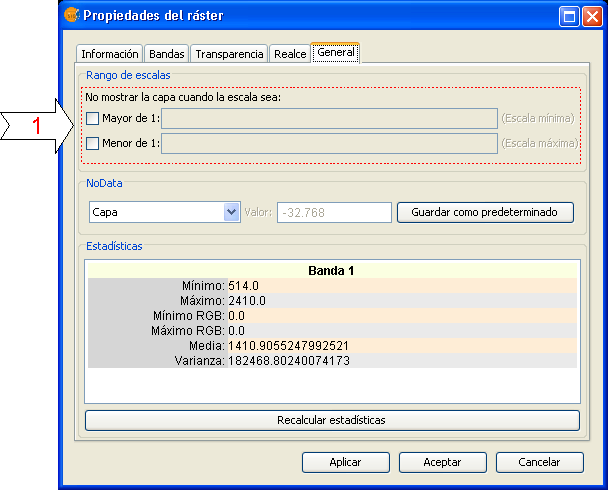
Image statistics
gvSIG can generate basic statistics over raster layers, which you can access through the option "Raster properties" that opens a dialog window with multiple tabs containing information about the selected raster layer. Select the "General" tab to see the layer statistics.
The dialog window "Raster properties" can be accessed in two ways: by right-clicking the raster layer in the table of contents, or from the raster properties icon in the toolbar:

Raster Properties icon
In this tab, you can see the layer statistics grouped by band. For each band the following information is shown:
- Minimum: Minimum value in the band.
- Maximum: Maximum value in the band.
- RGB Minimum: Minimum RGB value in the band.
- RGB Maximum: Maximum RGB value in the band.
- Mean: The average of all the values in the band.
- Variance: The amount of variation within the values in the band.
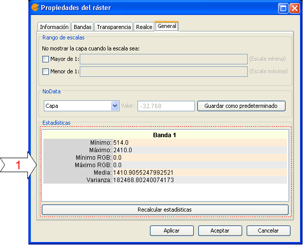
Raster properties window with image statistics
In case that the statistics are incomplete or erroneous, you can use the option "recalculate statistics" to regenerate the statistics.
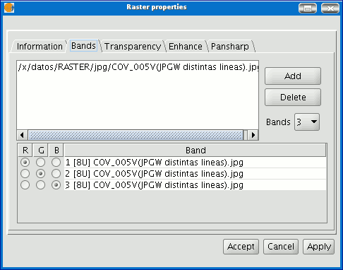
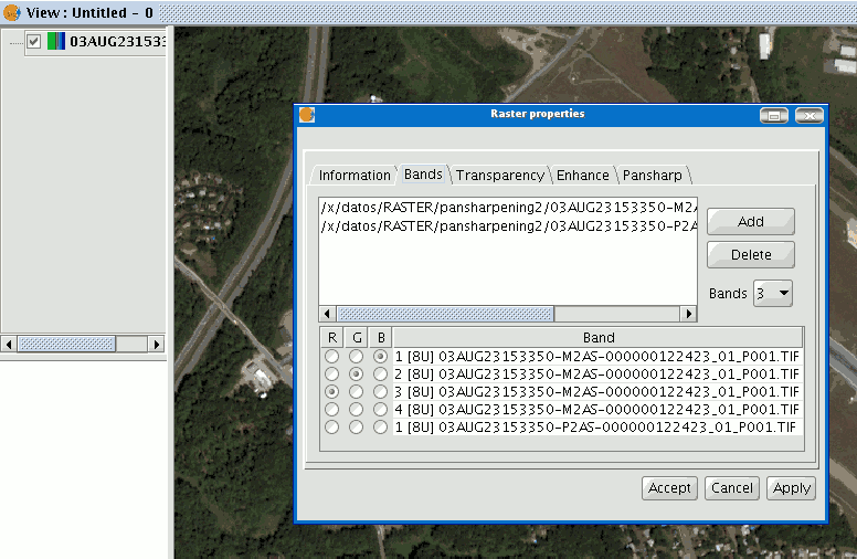
Bands and files selector
You can find information about the current raster layer through the option "raster properties", which opens a dialog with several tabs. To access the list of image bands and corresponding files, go to the tab "Bands".
The "Raster Properties" dialog can be accessed in two ways: by right-clicking on the raster layer in the TOC, or through the raster toolbar by selecting "Raster layer" on the left drop-down button and "Raster properties" on the drop-down button on the right. Make sure that the name of the raster layer for which you want to see information is displayed as current layer in the text box.

Raster properties icon
The "Bands" tab of the "Raster properties" dialog provides options to select band combinations for image display. The upper part of the dialog shows a list of files of which the image consists. You can add more files, but they must correspond to the same geographic area. This is useful when you need to load several files of the same sensor, each file representing a band.
In the lower part of the dialog you can select the display order of the bands. By default, the display order is assigned by the colour interpretation of the bands, if that information is available. With the option buttons, you can change the display order by marking the bands that should be displayed in red (R), green (G), blue (B) or alpha (A). When clicking on the "Save" button, the colour interpretation information will be saved and set as default for the image. This means that the next time that the image is loaded in gvSIG, the display order of the bands will according to the settings that you have saved.
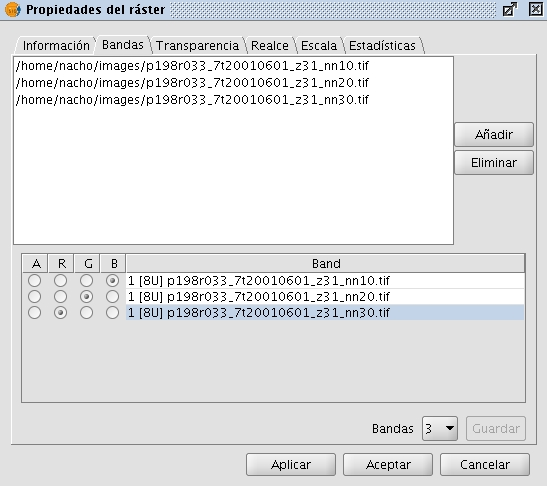
Raster properties. Band selection
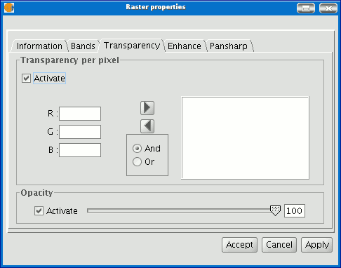
Transparency per pixel
You can find information about the current raster layer through the option "Raster properties", which opens a dialog with several tabs. To access the pixel transparency and opacity options, go to the tab "Transparency".
The "Raster Properties" dialog can be accessed in two ways: by right-clicking on the raster layer in the TOC, or through the raster toolbar by selecting "Raster layer" on the left drop-down button and "Raster properties" on the drop-down button on the right. Make sure that the name of the raster layer for which you want to see information is displayed as current layer in the text box.

Raster properties icon
The transparency options that are set here will only be applied to the current view (i.e. they will not be applied permanently to the image). The transparency will be calculated and applied each time when you zoom on the view. The transparency settings can be saved in the current project, and when the project is opened again, the transparency will be applied on the layer. However, if the same image is opened in another project, it will be displayed normally without the transparency settings.
The upper part of the "Transparency" tab of the "Raster properties" dialog shows a sliding bar labelled "Opacity". After activating the sliding bar by ticking the check box, you can modify the opacity of the whole layer by moving the slider. (Opacity is the opposite of transparency: if you set the opacity to 0%, the layer will be 100% transparent.)
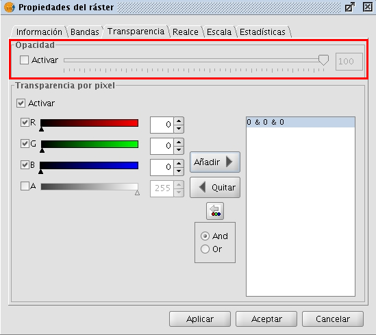
Set the transparency using the Opacity slider
The pixel transparency controls are located in the lower part of the "Transparency" tab. With these controls, you can apply transparency to pixels or a range of pixels depending on their RGB value. After activating the controls (by ticking the "Activate" check box) you can add specific RGB values to the list of elements through the "Add" button. Three values separated by the "&" or "|" symbol will be added as one item in the list; the three values correspond to the RGB value that will be set transparent. The values that are added are those that appear in the text boxes, the alpha value is optional. The information in these text boxes can be modified in three ways: typing the value directly by using the keyboard, moving the colour sliders on the left of the text boxes, or by clicking on the image in the view to select a specific colour value. This last option is activated with the button with the tooltip "Select RGB clicking on view". This will activate a crosshair cursor in the gvSIG view so that you can click on the image pixels and select the values for which you want to set the transparency.
If the line "255 & 0 & 0" is added to the list, this means that all pixels with the RGB values of 255 for red, 0 for green and 0 for blue (i.e. all pixels that are pure red) will be set transparent. The "&" symbol can be changed by the "And" and "Or" options. If "Or" is activated, the entries in the list will appear with the pipe symbol "|". The line "255 | 0 | 0" means that all pixels that have RGB values of 255 for red, or 0 for green, or 0 for blue will be set transparent. In this case many more pixels will be set transparent.
Set the transparency for specific pixel values
General components
Accessing raster functions from the toolbar
With the increase of image processing functions in the menu of gvSIG, the toolbar had to incorporate these Raster functions by grouping them as pull-down buttons.
As can be seen in the image below, when a view is selected, a control will appear at the right side of the toolbar.
Drop-down buttons for raster functions in the toolbar
The control has two drop-down buttons and a search combobox with the name of the current layer.
The buttons work as follows (see image below):
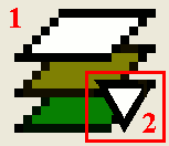
Raster drop-down button, with two zones (1 and 2)
- Clicking in this area will change the visible order of the button.
- Clicking the area with the pointing down arrow shows the menu of options.
Groups of raster functions
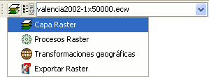
With the first drop down button you can access a set of grouped functions. For each group of functions, the individual functions within that group will be shown in the second button. Therefore, the functions that are available in the second button depend on the group of functions that is chosen with the first button.
Individual raster functions shown in the second drop-down button
In the image above, the individual functions from the second drop-down are shown while in the first drop-down button the function group "Raster layer" is selected.
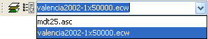
Combobox with the name of the current raster layer
The search combobox is used to select one of the layers in the TOC. When clicking on the arrow on the right, all the possible layers are shown.
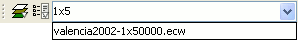
Search Combo to select a raster layer
You can write text in the combobox to filter the list of images (i.e. write "1x5" to show only layers that have these characters in their name).
Display of processing statistics when a new layer has been created
When processes that display a progress bar have ended, a statistics window with details of the process is usually shown.
Examples of such processes that launch statistics windows are Filters, Crop, Save As, etc.
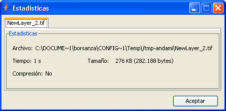
Statistics component
The statistics window shows the following information:
- File: Complete file path where the image has been stored.
- Time: The time that it took to complete the process.
- Size: File size on disk.
- Compression: Whether or not the image file has been compressed.
If you have generated more than one layer in the same process (as is the case when cropping images with multiple bands) the statistics window will display the information of each layer in a different tab.
The window can be closed by pressing the OK button.
Progress bar
When running processes that may take a considerable amount of time, a progress bar is shown.
The progress bar indicates that a process is running in the background and informs the user on the status of the process at any given moment and on how much time has elapsed since the process started.
In the image below, you can see a screenshot of the progress bar during a running process.
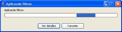
Progress bar component
The progress bar consists of several parts. The title indicates which process is running. Below the title, the current task that is being processed is indicated as well as the percentage of the process that has been completed.
The progress bar contains two buttons. To see more details, you can click the left button, after which the dialog is enlarged to display additional information as in the screenshot below.
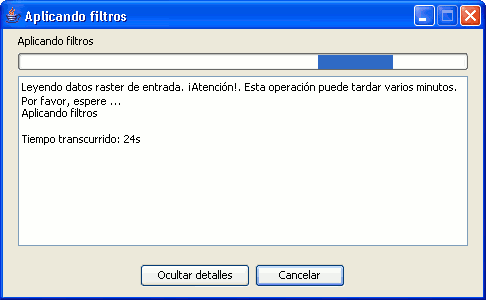
Progress bar with details
The additional information includes a list of tasks that have been performed and an indication of how much time has elapsed since the process was started.
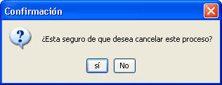
Confirmation message: are you sure you want to cancel this process?
If you want to cancel a process, you can click on the "Cancel" button on the right. A message will appear to prompt for confirmation. Clicking on the "Cancel" button does not always guarantee that the process is stopped immediately. Depending on the process, certain tasks might be needed to reverse the process and return to the previous state.
Table control
The table control component is used to represent data in tabular form and allows you to edit the data.
The possibilities are:
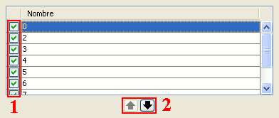
Table control components (1 and 2)
- Selection of rows in the table.
- Reordering the rows. Click on the arrow buttons to move a selected row up or down.
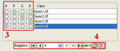
Table control components (3 and 4)
Choose a unique property for every row. In the example above, a band is allocated for each layer.
Typical table controls, as shown in the example at the bottom of the table. From left to right:
- Select the first row.
- Select the previous row.
- Drop down to select a particular row.
- Select the next row.
- Select the last row.
- Create a new row.
- Delete the selected row.
- Delete all rows from the table.
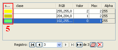
Table control components (5)
- In the table control, besides being able to edit anything if editing is enabled, you can also change the color by clicking on it.
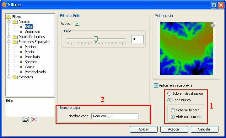
Output selector
The output selection control is used to create new layers.
In this example the output selection control is shown in the lower right corner of the dialog (1):
Output file selection
The selector consists of two components:
- For the output image, you can choose whether to apply the filters over the image in the current view (only for display) or save the output as a new layer.
- The option "Only on visualization" does not change the original layer, but will apply the list of filters when drawing and re-drawing the view. This option is faster when the image is very large (as the filters are only applied to the current view, not to the whole image), but it slows down the drawing and re-drawing of the view.
- The option "New Layer" will apply all the filters to the image and save the output to a new layer. This is faster when the image size is medium or small and the applied changes are considerable. The generation of the new layer will take some time, but then the displaying is as fast as it would be without the filters.
Both options have advantages and disadvantages, and it is up to the user to decide which option to choose.
- When selecting the option "New Layer", a second option control is enabled in which you can choose whether to save the layer to disk (Create file) with a file name specified in the text box (2), or to create a temporary gvSIG layer (Open in memory).
The new layer will be added to the view, and the TOC will show the layer name as specified in the text box.
** Note: The temporary working space of gvSIG is cleaned automatically, so any temporary layers will be deleted when exiting the application.
Previewing the output
A preview is usually shown for functions that require extensive processing. It is usually located in the upper right corner of the dialog as shown in the following example:
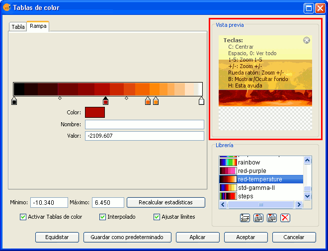
Component 'Preview'
The preview gives only an indication of how the final output will look like. Since only a minimum amount of data is used to generate the preview, the final result may be different.
The following options are available for preview windows:
- Move the image with the left mouse button.
- Center the image in the preview by pressing the C key.
- Zoom out to see the whole image with the space bar or 0
- Predefined zooms with keys 1 to 5. 1 gives a 1/1 zoom.
- Zoom with the mouse wheel or arrow keys + and -.
- Show a grid on the background to view images with transparency by pressing the B key.
- Access the help function by pressing the H key or clicking on the question mark in the upper right corner of the preview window.
The access to these preview functions through the shortcut keys only works when the focus is on the preview window, after clicking on it with the mouse.
For different types of functionality, the preview may appear with a different default zoom level. For example, the preview of colour tables is shown as completely zoomed out so that the effects on the whole image can be previewed.
Table of contents (ToC)
Table of contents
The “Table of Contents” is the area used to list the different layers which make up the cartographic information.
A check box next to each layer indicates whether it is "visible” or not.
Remember that an active layer is not the same as a "visible" layer. When a layer is “active” it is highlighted compared to the other layers included in the “Table of contents”. When a layer is activated, gvSIG is notified that the elements of this layer can be worked with.
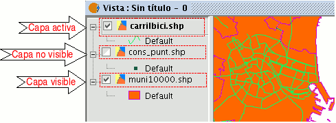
The order of appearance of the layers in the “View” is important because it ties in with the display order. Layers made up of text elements, points and lines are placed at the top whilst the polygonal layers and images which make up the background of the view are placed at the bottom.
To move the layers in the ToC, place the cursor over them, left click on the mouse and drag the layer to the required position.
The layers in the ToC can also be selected by using the Control and CAPS keys.
Grouping and ungrouping layers
From version 0.4 onwards, gvSIG allows several layers to be grouped together. This is useful because it means a large number of layers can be kept in the ToC without taking up a lot of space. This option also allows operations to be carried out on all the layers that make up a group at the same time. To group a set of layers together, select the layers, click and hold down the CAPS key and right click on the mouse on any of the layers and select the “Group layers” option.
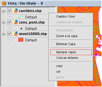
The following dialogue window appears and a name for the new grouping can be input.
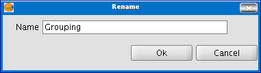
When the name of the new grouping has been input, it appears in the ToC as shown below.
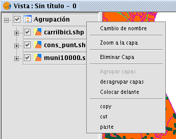
To undo a grouping, right click on the grouping so that the contextual menu appears. Select the "Ungroup layers" option.
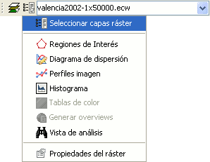
Select raster layer
Raster layers can be selected through the raster toolbar by selecting the option "Raster layer" on the left drop-down button and "Select raster layers" on the drop-down button on the right.

Select raster layer icon
When multiple raster layers have been loaded into the view, you can select one of those as current layer. By clicking on one of the layers in the TOC, the layer will be selected and its name will appear as current layer in the drop-down text box of the toolbar.
Properties of a view in gvSIG
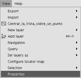
To access the properties window of a view, go to the “View” menu and select “Properties”.
The properties you wish your view to have can be configured via the following window.
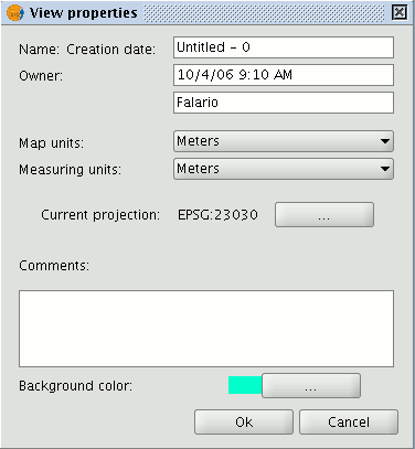
If you click on the “Current projection” button, a new window will appear in which the view’s datum, projection and time zone can be selected.
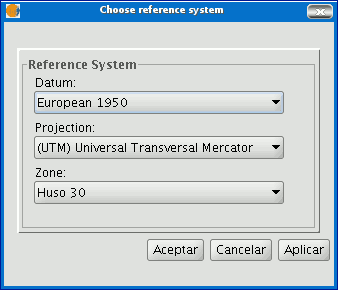
If you click on the pull-down menus, the different options available for each element in the reference system are shown. If you make any changes, click on “Apply” and then “Ok”.
When you have configured the view’s properties, click on “Ok”.
Maps
Introduction
“Map” type documents allow you to design and combine all the elements you wish to have on a printed map.
Accessing maps
You can access “Map” type documents via gvSIG's "Project manager".
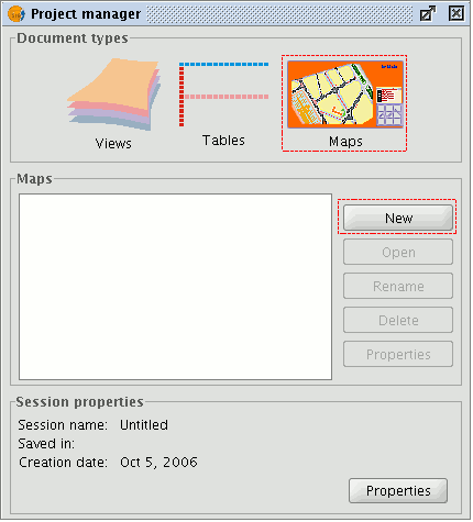
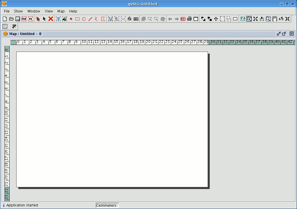
Click on “New” to create a new map. When you have created the document (it will appear by default as “Untitled– 0”), you will be able to insert elements, rename the map, delete it or access its properties and modify them. When the map is open, it will appear in gvSIG as shown below:
Map properties
You can access the map properties window from the “Project manager” by clicking on the “Properties” button or from the view by going to the “Map” menu and then to “Properties”.
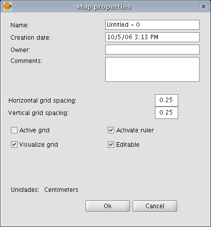
You can use the properties window to rename the map, change its creation date, add an owner and comments. You can select some default characteristics by activating the corresponding check boxes:
- Active grid: Activating the grid means that any element inserted in the map will be adjusted to the grid. Remember the following two points if you enable “Active grid”:
- The horizontal and vertical grid spacing defines the distance between the different points which make up the grid. This can be modified by inserting new values in the text boxes.
- Output size of the chosen document (A2, A3, A4,...). The zoom tools may need to be used to be able to view the grid when you open the document.
- Visualise grid: If this box is disabled, the grid will not be viewed when you open the newly created document.
- Enable ruler: By enabling this check box a ruler appears which can be used as a drawing aid.
- Editable: If you do not enable this option, the objects that make up the map will be blocked, thus preventing modifications.
Copying layers in gvSIG
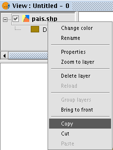
You can also use gvSIG to copy documents and create copies of the layers you are working with in your view. Firstly, select the layer in the ToC and right click on it. A new menu appears. Select the “Copy” option.
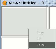
You can paste the layer you wish to copy in the same view as the one you are working with or in a different view, either in the same project or in a different one.
N.B.: Remember that currently if you modify the layer, these changes will be reflected in all the copies.
If you wish to “Paste” the layer, right click on the point you wish to paste the new copy and select the “Paste” option.
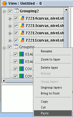
N.B.: You can use this method when working with layer groups.
If you create a layer group, place the mouse pointer over the group name and go to the “Copy” option, you can “Paste” the whole layer group in the same way as you would with an individual layer.
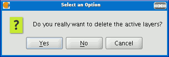
Deleting layers
To permanently remove the active layers from the view, right click on the layer in the ToC and select the “Delete layer” option.
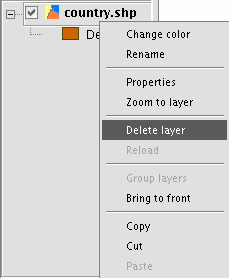
A confirmation dialogue appears.
Exporting to image
This option allows you to convert the active view into an image or raster file.
Select the “View” menu then go to “Export/Image”.
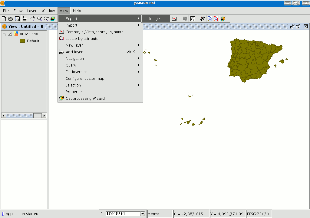
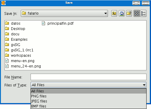
When you have selected the tool, a new window appears which you can use to edit the name of the image to be saved and the type of file (jpg, png...) you wish to save it in.
When you have saved the image, you can recover it from gvSIG by going to the “Add layer” tool and searching for a “gvSIG Image Driver” file type.
Use the ToC to check that the exported image is a raster layer by accessing its properties (right click on the layer in the ToC and then go to “Raster properties”).


